The Challenges faced by Small and Medium Enterprises – Food Processing, Ghana
If you are looking 100% error-free Best Assignment Writing Service in Australia, then we are here to assist you. Our team of professional and skilled expert writer is available 24×7 to provide you Online Assignment Help at any time. Most students get in touch with us for Case Study Writing Help and Dissertation Writing Help. Contact us now and get instant solution on Analyzing Financial Risks in Small and Medium Enterprises Assignment as soon as possible.

Assignment Details:-
- Topic : Research Methodology
- Words : 5000
- Deadline :As Per Required
Analyzing financial risks in small and medium enterprises: evidence from the food processing firms in selected cities in Ghana
Introduction
The financial-growth nexus (Schumpeter, 1911) argues for the critical role of finance in the growth of an economy including its agents such as the firm. The theory postulates that finance is critical in promoting innovations; and that economies with better financial infrastructure will grow faster (Jayaratne and Strahan, 1996; Hacievliyagil and Eksi, 2019). This implies access to finance is a key determinant of the firm’s growth (Regasa et al., 2019). This means it is imperative for the owner/manager to evaluate the nature of finance available to them, analyzing their potential risks and how such risks impact the firm. Due to their nature, SMEs potentially face moral hazards by being wrongly categorized by lenders and financial institutions. Lenders may misclassify SMEs seeking credit to manage their financial institution’s default rate. Evidence from studies (Nguyen et al., 2006; Ilyas, 2019) points to the difficulties of FIs in ascertaining the true quality of an owner–manager in financial transactions including credit granting and provision of financial services.
Furthermore, FIs have often contemplated the information gap based on information asymmetry theory. This theory argues that in most cases with credit-seeking transactions, the owners/managers do conceal relevant information lenders. Meanwhile, such information tends to affect the terms and conditions of the loan contract between the parties. The result has been an adverse selection by the lenders. Several studies have argued in this direction (Motta and Sharma, 2019; Gou and Huang, 2019; Moyi, 2019) without looking at the tendency for the owner/managers to suffer from adverse selection due to non-disclosure of credit information. There is a tendency for lenders to withhold information from their clients. Extant studies (Yen et al., 2019; Ol´ah et al., 2019; Haniff et al., 2017; Rao et al., 2017; Bbenkele, 2007) report owner–manager complaint about lack of transparency in credit granting contract with FIs. Lenders have often relied on their previous experience and transactions with SMEs in setting credit granting criteria. In many circumstances, although the business characteristics of the SME have changed, lenders’ criteria often remain the same. This may pose a financial risk for the owner /manager as such perception tends to influence the cost of credit. Besides lenders, different actors within the business ecosystem expose the owner/ manager to the different types of financial risks.
Stakeholders’ theory outlines several other actors and groups that engage in a financial transaction with the business. The tenet of this theory is that businesses have actors whose actions affect the business or the firm’s actions affect them. Among these actors are customers, suppliers, employees, auditors, stock and bondholders, banks, middlemen, communities, competitors and managers (Freeman, 1984; Jones, 1995; Walsh, 2005; Freeman et al., 2010). Every aspect of the business–stakeholder interaction creates a financial relation and risks between the firm and the particular actor. For instance, the customer and their purchasing power could create a potential financial risk for the business. Financial relation is also created in the supplier–owner/manager interaction as well as the middleman. The tenets of the stakeholder theory are how the firm interacts with people and organizations taking into consideration the interest and power of these actors. Such interest and power have the potential to expose the business to hazards at different levels and ultimately various forms of risks (Jenkins, 2004; Yiannaki, 2012) and financial risks in particular.
The subject of financial risks in small businesses has become a subject of interest to scholars in emerging countries due to the critical role of such economic actors in development.
As a part of the broader concept of business risks, financial risk concentrates on uncertainties associated with funds flow into and out of the business (Ekaterina and Thielmann, 2020). It is the unexpected variations in prices and its impact on future cash flows of a firm (Jorge and Augusto, 2011). Yang et al. (2020) opine that financial risk for SMEs is an estimate of their future credit status. Yet, Gabriel and Baker (1980) define it as the risk of not being able to meet prior claims with inflows generated by the business. These empirical studies focused on cash flows. There are financial risks associated with any of the business transactions with stakeholders that impact on business operations. Meanwhile, the most serious risks are economic (Kozak and Danchuk, 2016) and financial risks (Bel´as et al., 2018; Cipovov´a and Dlaskov´a, 2016; Neacsu et al., 2018). As Ol´ah et al. (2019) and other similar authors opined, these risks are often difficult to deal with by the owner/managers of SMEs. An investigation into financial risks in SMEs is essential because of developments in the sector where businesses are failing due to poor cash flows, poor debt management (Asgary et al., 2020), inappropriate credit-granting policy (Khan, 2020; Wasiuzzaman et al., 2020) or use of the inappropriate financing methods (Utomo et al., 2020; Shaverdi et al., 2020) and unsuitable inventory practices (Xu and Li, 2019). Understanding their level of knowledge and how they respond to financial risks would reduce their exposure and ultimately their mitigation strategies. It is expected the appropriateness of their mitigation would help reduce the financial loss they face.
Stakeholders’ interest and power have the potential of exposing businesses to different forms of financial risks impacts on their business performance. However, previous research has not looked at the perception of owners/managers about risk, especially financial risks, and how such risks affect firm performance. The paper was motivated by the need to analyze the financial risk perception of owners/managers and to link such perception to the performance of their ventures. The rest of the paper is divided into five parts. Part two was devoted to the review of the literature. The research method was discussed in the third part. The analysis of results and discussion was in the fourth part and the practical and policy implications were in the final part.
Literature Review
Kundid and Ercegovac (2011) found that in comparison to large enterprises, SMEs continuously encounter higher borrowing costs, upon which this discrepancy enlarges in the aftermath and presence of financial crisis. Furthermore, the market cleaning of the SMEs’ credit applications evolves on the level of higher interest rates. This comes at the backdrop of the perception that SMEs are risky to deal with. Owusu (2019), Abimbola and Kolawole (2017) argue that about 60% of SMEs fail within the first five years due to inadequate financial management skills. Similarly, Morgan et al. (2015) observed that the failure and poor performance of SMEs to the challenges of financial management and inventory. Such situations if not properly managed could be the basis for financial risks in the firm.
Meanwhile, previous studies conducted on financial risk and firm performance focused on the banking sector (Dimitropoulos et al., 2010; Al-Khouri, 2011; Ruziqa, 2013; Abdallah et al., 2014) with few of them focusing on SMEs (Noor and Abdalla, 2014), thus creating a research gap a case for the food processing sector. Noor and Abdalla (2014) argued that SMEs are exposed to various financial risks including exchange rate risk, liquidity risk, interest rate risk, credit risk, the market risk with inconsistent influence on firm performance. In the case of food-processing SMEs in developing countries they depend largely on imported tools and technology, hence the tendency for their performance to be negatively affected by exchange rate risks. Jones et al. (2018) suggest technology-focused entrepreneurship development around major cities in Africa to foster their success. A study by Boermans and Willebrands (2011) found a significant negative effect of financial risk on profit levels. The finding was supported by Tafri et al. (2009), Dimitropoulos et al. (2010), Qin and Pastory (2012). Van Greuning and Bratanovic (2009) asserted that liquidity risk poses serious threats to SMEs’ performance levels, thus are negatively correlated. Yusuf and Dansu (2013) also examined the relationship between business risk and sustainability of SMEs using Chi-square. They discovered that business risks affect performance levels. However, Chi-square is highly sensitive to sample size. Thus as sample size increases, absolute difference reduces and become a smaller percentage of the expected value. The reverse occurs when the sample size decreases. This situation tends to affect the predictive power of the model.
A study by Abeyrathna and Kalainathan (2016) examined the relationship between financial risk and SMEs’ performance in the Anuradhapura district. Focusing on 30 purposively sampled SMEs from 5,000 registered SMEs, the study found no significant relationship between financial risk and performance. However, the question is whether the sample size was representative of the population selected. Similarly, Ombworo (2014) investigated the effect of liquidity risk on performance (profitability) of SMEs in Kenya. Using the descriptive research design while adopting both descriptive and quantitative analytical tools, the study found a positive but no significant effect of liquidity risk on SMEs’ performance. Noor and Abdalla (2014) found financial risks impact on financial performance, although the direction of the effect was not indicated. Offiong, Udoka, and Bassey (2019) found a negative but insignificant relationship between financial risk and SMEs’ performance in Nigeria. However, they found liquidity risk, exchange rate risk, inflation and interest risks to significantly but negatively influence SMEs’ performance levels. Moyi (2019) discovered that lending to small businesses does not affect credit and insolvency risk in lending institutions. This is because there may be several factors that could lead to the insolvency of a lending institution such as governance, macroeconomic factors including regulations (Lindsay and Butt, 2020; Huhtilainen, 2020).
It could, therefore, be deduced that previous studies on SMEs have revealed inconsistent findings with some revealing significant relationships (Boermans and Willebrands, 2011; Tafri et al., 2009; Qin and Pastory, 2012; Yusuf and Danso, 2013), whereas others (Ombworo, 2014; Abeyrathna and Kalainathan, 2016; Offiong et al., 2019) found no significant relationships between financial risk and SME’s performance. Studies including Christopoulos and Barratt (2016), Bet´akov´a et al. (2014), Mentel et al. (2016) and Ol´ah et al. (2019) found financial risks impact on firm performance. However, they did not indicate the direction of the effect. O€zbug˘day et al. (2019) are among studies that highlight SMEs’ performance and compliance.
They submit that compliance with environmental standards through resource efficiency investments can serve as a quality strategy for an SME to increase its sales. Meanwhile, Liu (2020) suggests that it is essential for firms to have adequate financial resources to implement proactive environmental programs. Other studies, such as Jones et al. (2018), cite the need for technology-focused entrepreneurship to boost entrepreneurial activity. This suggests the critical role of technology and technology risks in the survival of SMEs. These inconsistencies presented research gap for further investigation into this phenomenon, particularly food processing industry with huge economic potential for the economy of Ghana.
An interesting debate in the literature is the impact of social responsiveness on the performance of SMEs. Boutin-Dufresne and Savaria (2004) observed the adoption of corporate social responsibility codes of conduct could reduce the overall business risk of a firm, and even increase its long-term risk-adjusted-performance. K€olbel et al. (2017) concluded corporate social irresponsibility exposes the firm to financial risk via media coverage. It could be deduced from the extant studies three key issues required attention. These included the lack of consensus on the effect of financial risks on firm performance; the lesser attention of previous studies on the food processing sector; and inadequate literature on financial risks and firm performance in SMEs in Ghana. Besides, the paper employs the two-stage PLS-SEM hierarchy construct modeling in its analysis, different from previous studies. The study, therefore, addresses these gaps by examining the effect of financial risk on the performance of SMEs in the fruit processing sector in Ghana.
Research Methods
The study employed a quantitative explanatory approach. The population consisted of small firms in the food processing sector. In a preliminary exploratory study, over 2000 of such firms were identified in the selected cities. The source of data for this part included Association of Ghana Industries (AGI), National Board for Small Scale Industries (NBSSI) and other databases. The basic criteria for inclusion were that the firm should be registered and fall into SMEs as defined by the Ghana Statistical Service. A sample size of 214 was selected using the Bartlett et al. (2001) sample size determination formula. However, through the application of the Nyquist sampling theorem, a sample size of 224 was used (Nyquist, 2002). As Nyquist suggests, sampling up to twice the minimum original size helps avoid aliasing, helping to obtain enough samples to capture the spatial or temporal variations in data.
The sampling procedure followed a three-step process. First was the creation of the sampling frame from the identified databases (AGI, NBSSI etc.) from the selected cities. This gave a total of 2000 firms. The cities were selected based on their qualification as major industrial hubs in the country. Second, identification numbers were assigned to the businesses obtained from the database of food processors. MS Excel was, then, used to generate and select a randomized sample of respondents based on the identification number assigned to the business. The databases used in the participant selection contained the details of the businesses that were used to reach out to the owner/managers. One reason why food processing businesses locate in the urban centers is access to market and infrastructure compared to the rural areas. The study sought to understand how financial risk perception of managers predicts firm performance. The proxies included financial risks arising from operational, market and technology risks. The dependent variable (performance) was measured using indicators including financial performance, compliance, social and resource efficiency performance.
Data used in the study were obtained mainly from the primary source. The main instrument for data collection was the questionnaire. The questionnaire was made up of an 11-point Likert-like scale with 0 (no agreement) to 10 (high agreement). This scale permitted respondents to rate the series of questions used as the constructs (Sekaran and Bougie, 2003; Agyapong and Attram, 2019). The Likert scale has been employed in several studies to study behavior that cannot directly be measured (Willits et al., 2016; Joshi et al., 2015; Agyapong and Attram, 2019). Using a Likert-like scaled questionnaire, data were obtained from 214 managers of small businesses.
Measurement of variables
The study analyzed financial risks in SMEs in the food processing sector. It also examines how such risks affect their performance. The nature of risks and performance were defined and measured as follows:
Financial risks indicators
The components of the financial risks were made up of operational, market, technological, credit and liquidity risks:
- Operational risks (op_risk): It is the chance of loss emanating from people, systems, procedures and external events. This was measured with constructs related to legal, compliance, reputational and people risks.
- Credit risks (cr_risk): This is a measure of the uncertainty associated with debtors defaulting in payments. Among the issues considered here included credit default risk, settlement risk, concentration risk, recovery risk and credit detection risk.
- Liquidity risks (li_risks): This included risks associated with inadequate liquid assets. Items considered here included asset liquidity risk, inability to meet short-term financial requirements and refinancing risks.
- Market risks (mk_risk): This is looked at as the chance of loss arising from increases in interest rates, poorer liquidity conditions and a decline in credit quality. It was measured using constructs related to interest rate, currency, raw materials, end-product, current monetary policies and economic performance risks.
- Technology risks (tech_risk): This was measured using constructs including risks from damages to operating systems; cost associated with acquiring technological infrastructure; exposure to cyber attacks or data breaches; telecommunication and connectivity issues and data integrity.
Performance Measures
The performance was defined as the ability to create acceptable outcomes and actions (Eniola and Entebang, 2015). There were some constructs used for measuring each of the variables of performance. The proxies for performance followed the work of Selvam et al. (2016). Financial performance (fperf) constructs included an increase in profitability due to improved sales from productive activities of the firm (Henri, 2006; Nasiri, 2020). Compliance (cperf) constructs were the firm’s preparedness and response to legislations and policies regulating the food processing sector. Furthermore, the social performance (sperf) was the firm’s response to social and community needs. This includes the firm’s contribution to community development and support. The resource efficiency (reperf) was operationalized as how efficiently the firm uses resources. This has to do with its sustainability practices.
Also Read:- Free Finance Assignment Sample
Data Analysis
Data collected was analyzed within the partial least squares’ structural equation modeling (PLS-SEM) framework backed by the stakeholder theory. This method integrates complex path models with latent variables. It combines the features of factor analysis and multiple regressions that help examine the relationship between endogenous and exogenous variables (Bagozzi and Fornell, 1982; Genfen and Straub, 2000; Hair et al., 2006; Hair et al., 2017b, c; Agyapong and Attram, 2019). This technique is appropriate where studies are limited by non- normal data and small sample size. It is used in nominal, ordinal and interval scales of measurements. It supports formative measured constructs (Hulland, 1999). It permits the mixing of categorical, discrete and continuous variables (Civelek, 2018). Babin et al. (2008) positioned that the PLS-SEM uses confirmatory approach (hypothesis-testing) to examining structural theory in any given situation.
R€onkk€o and Evermann (2013) added that PLS-SEM is a complex technique capable of analyzing relationships between/among constructs under study. According to Hair et al. (2017b, c), this technique has more powerful and rigorous statistical processes to handle complex models. It was, therefore, relevant for analyzing studies of this nature. It is to note that the study’s analysis of its five models was based on this analytical technique. The models were used to predict the relationship between the variables:
- Model 1: financial risk and performance using the higher-order constructs.
- Model 2: compliance performance predicted by financial, social and resource efficiency.
- Model 3: financial performance explained by compliance, social, and resource efficiency.
- Model 4: compliance, financial and resource efficiency explain social performance.
- Model 5: effect of compliance, financial and social performance elements on resource efficiency.
An exploratory factor analysis was performed to uncover the underlying structure of the financial risk variables. In the process of conducting the analysis, there was a need to examine the appropriateness of the dataset. This was done by employing the Kaiser–Meyer–Olkin (KMO) measure of sampling adequacy and Bartlett’s test for sphericity (Table 1). The KMO test revealed an adequacy value of 0.897 which was higher than the minimum benchmark value of 0.7 (Pallant, 2011). Also, Bartlett’s test for sphericity (χ2 5 7700.437; df 5 1,378) had a p-value which was less than the 0.01 benchmark value, meaning the responses of the respondents revealed an unidentical correlation matrix. The outcomes of these two tests validate the use of the exploratory factor analysis (Pallant, 2011).
The total variance explained in Table 2 showed that 25 components of the extracted risk factors were reduced to six components with 76.14% as its cumulative variance explained of the total variance. These six components came as a result of the benchmark eigenvalue of 1, meaning components with eigenvalues less than this benchmark were dropped. Also, a scree plot was plotted that confirms this outcome (see Appendix 4).
| Kaiser–Meyer–Olkin measure of sampling adequacy | 0.881 | ||
| Table 1. | Bartlett’s test of sphericity | Approx. Chi-Square | 3678.114 |
| KMO and | Df | 300 | |
| Bartlett’s test | Sig | 0.000 |
| Component | Total | % of variance | Cumulative % | Total | % of variance | Cumulative % |
| 1 | 9.894 | 39.576 | 39.576 | 9.894 | 39.576 | 39.576 |
| 2 | 3.623 | 14.491 | 54.067 | 3.623 | 14.491 | 54.067 |
| 3 | 2.087 | 8.350 | 62.417 | 2.087 | 8.350 | 62.417 |
| 4 | 1.194 | 4.777 | 67.194 | 1.194 | 4.777 | 67.194 |
| 5 | 1.151 | 4.605 | 71.799 | 1.151 | 4.605 | 71.799 |
| 6 | 1.084 | 4.336 | 76.135 | 1.084 | 4.336 | 76.135 |
| 7 | 0.807 | 3.229 | 79.364 | |||
| 8 | 0.686 | 2.742 | 82.106 | |||
| 9 | 0.506 | 2.024 | 84.130 | |||
| 10 | 0.449 | 1.795 | 85.925 | |||
| 11 | 0.436 | 1.744 | 87.669 | |||
| 12 | 0.380 | 1.519 | 89.188 | |||
| 13 | 0.348 | 1.391 | 90.579 | |||
| 14 | 0.337 | 1.349 | 91.928 | |||
| 15 | 0.306 | 1.222 | 93.150 | |||
| 16 | 0.292 | 1.169 | 94.319 | |||
| 17 | 0.216 | 0.864 | 95.183 | |||
| 18 | 0.204 | 0.817 | 96.000 | |||
| 19 | 0.195 | 0.781 | 96.781 | |||
| 20 | 0.176 | 0.704 | 97.484 | |||
| 21 | 0.158 | 0.633 | 98.117 | |||
| 22 | 0.154 | 0.617 | 98.734 | |||
| 23 | 0.119 | 0.475 | 99.209 | |||
| 24 | 0.102 | 0.408 | 99.617 | |||
| 25 | 0.096 | 0.383 | 100.000 | |||
Note(s): Extraction Method: Principal Component Analysis
The rotated component matrix serves as a technique for retaining factors which are rotated to establish a simple structure. The rule of thumb was that factors with factor loadings greater than 0.4 were retained. The Varimax rotation was employed because the variables were uncorrelated. Factors with higher factor loadings were regarded to have a greater contribution. Even though 6 components were built, 4 out of the 6 were market risk factors (MR) and the last two were operational risk (OR) and technical risk (TR). This is seen in Table A1 (Appendix 1).
For the performance measures, the KMO test revealed an adequacy value of 0.897 which was higher than the minimum benchmark value of 0.7 (Pallant, 2011). Also, Bartlett’s test for sphericity (χ2 5 7700.437; df 5 1,378) had a p-value which was less than the 0.01 benchmark value, meaning the responses of the respondents revealed an unidentical correlation matrix. The outcomes of these two tests validate the use of the exploratory factor analysis (Pallant, 2011) (see Table 3).
The total variance explained Table 4 showed that 53 components of the extracted performance factors were reduced to 8 components with 74.04% as its cumulative variance explained of the total variance. These eight components came as a result of the benchmark eigenvalue of 1, meaning components with eigenvalues less than this benchmark were dropped. Also, a scree plot was plotted that confirms this outcome (see Appendix 5).
| Component | Total | % of variance | Cumulative % | Total | % of variance | Cumulative % |
| 1 | 18.602 | 35.099 | 35.099 | 18.602 | 35.099 | 35.099 |
| 2 | 8.913 | 16.817 | 51.915 | 8.913 | 16.817 | 51.915 |
| 3 | 3.574 | 6.743 | 58.658 | 3.574 | 6.743 | 58.658 |
| 4 | 2.677 | 5.050 | 63.708 | 2.677 | 5.050 | 63.708 |
| 5 | 1.671 | 3.153 | 66.862 | 1.671 | 3.153 | 66.862 |
| 6 | 1.529 | 2.885 | 69.747 | 1.529 | 2.885 | 69.747 |
| 7 | 1.209 | 2.281 | 72.028 | 1.209 | 2.281 | 72.028 |
| 8 | 1.067 | 2.014 | 74.042 | 1.067 | 2.014 | 74.042 |
| 9 | 0.982 | 1.852 | 75.894 | |||
| 10 | 0.957 | 1.805 | 77.700 | |||
| 11 | 0.838 | 1.581 | 79.281 | |||
| 12 | 0.789 | 1.488 | 80.769 | |||
| 13 | 0.760 | 1.434 | 82.204 | |||
| 14 | 0.735 | 1.387 | 83.591 | |||
| 15 | 0.573 | 1.082 | 84.672 | |||
| 16 | 0.554 | 1.046 | 85.718 | |||
| 17 | 0.542 | 1.023 | 86.742 | |||
| 18 | 0.531 | 1.003 | 87.744 | |||
| 19 | 0.483 | 0.911 | 88.656 | |||
| 20 | 0.438 | 0.826 | 89.481 | |||
| 21 | 0.413 | 0.779 | 90.261 | |||
| 22 | 0.371 | 0.700 | 90.960 | |||
| 23 | 0.343 | 0.647 | 91.607 | |||
| 24 | 0.335 | 0.632 | 92.239 | |||
| 25 | 0.309 | 0.582 | 92.821 | |||
| 26 | 0.289 | 0.545 | 93.367 | |||
| 27 | 0.282 | 0.533 | 93.899 | |||
| 28 | 0.253 | 0.478 | 94.377 | |||
| 29 | 0.235 | 0.444 | 94.821 | |||
| 30 | 0.228 | 0.431 | 95.252 | |||
| 31 | 0.220 | 0.416 | 95.667 | |||
| 32 | 0.198 | 0.375 | 96.042 | |||
| 33 | 0.197 | 0.373 | 96.415 | |||
| 34 | 0.177 | 0.335 | 96.749 | |||
| 35 | 0.159 | 0.300 | 97.049 | |||
| 36 | 0.154 | 0.291 | 97.340 | |||
| 37 | 0.140 | 0.265 | 97.605 | |||
| 38 | 0.135 | 0.254 | 97.859 | |||
| 39 | 0.125 | 0.235 | 98.094 | |||
| 40 | 0.120 | 0.227 | 98.321 | |||
| 41 | 0.110 | 0.207 | 98.528 | |||
| 42 | 0.093 | 0.175 | 98.703 | |||
| 43 | 0.086 | 0.163 | 98.866 | |||
| 44 | 0.079 | 0.148 | 99.014 | |||
| 45 | 0.076 | 0.143 | 99.158 | |||
| 46 | 0.074 | 0.140 | 99.298 | |||
| 47 | 0.070 | 0.131 | 99.429 | |||
| 48 | 0.065 | 0.123 | 99.552 | |||
| 49 | 0.062 | 0.118 | 99.670 | |||
| 50 | 0.053 | 0.100 | 99.770 | |||
| 51 | 0.050 | 0.094 | 99.863 | |||
| 52 | 0.042 | 0.079 | 99.943 | |||
| 53 | 0.030 | 0.057 | 100.000 |
Note(s): Extraction Method: Principal Component Analysis
The rotated component matrix serves as a technique for retaining factors which are rotated to establish a simple structure. The rule of thumb was that factors with factor loadings greater than 0.4 were retained. The Varimax rotation was employed because the variables were uncorrelated. Factors with higher factor loadings were regarded to have a greater contribution. Even though eight components were built, four out of the eight were financial performance factors (FP); two were social performance factors (SP) and the remaining two (4) were CP, resource efficiency performance (REP) (Table A2 – Appendix 2).
Model 1
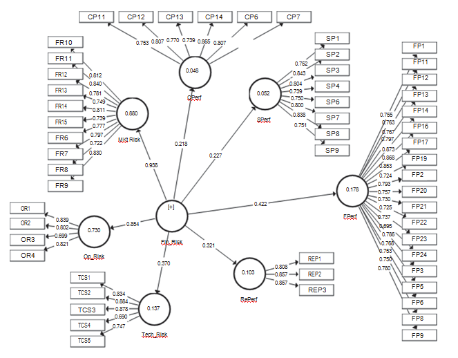
The financial risk was modeled to reflect three main attributes in the context of this study including market risk, operational risk and technology risk. Each of these separate risks was also measured with a set of indicators. Accordingly, financial risk was modeled as a second- order construct while market risk, operational risk and technology risk were measured as the first-order construct. The reason for such an approach was in line with Polites et al. (2012) and Hair et al. (2017b, c), who mentioned that broader constructs help to capture all possible measures in the construct’s domain and also higher-order constructs helps to reduce the number of relationships to achieve model parsimony.
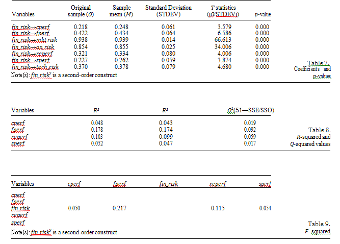
From a measurement theory perspective, op_risk, cr_risk, li_risks, mk_risk, and tech_risk can be considered as reflections of financial risk (Cabedo and Tirado, 2004; Deng, 2020; Yang, 2020), thereby implying the use of a reflective-reflective higher-order construct, since each of the lower-order components is measured reflectively. In the following, the estimation of the higher-order constructs is illustrated using the (extended) repeated indicators approach. The assessment of the lower-order components draws on the standard reliability and validity criteria for reflective measurement models as documented in Hair et al. (2017a), Latan and Noonan (2017) and Sarstedt et al. (2017). The results in Table 5 show the measures of mkt_risk yield satisfactory levels of convergent validity in terms of average variance extracted (AVE 5 0.619) and internal consistency reliability (composite reliability ρC 5 0.942; Cronbach’s alpha 5 0.931; ρA 5 0.933). Similarly, the measures of op_risk exhibit convergent validity (AVE 5 0.627) and internal consistency reliability (composite reliability ρC 5 0.870; Cronbach’s alpha 5 0.800; ρA 5 0.810). Also, the measures of tech_risk exhibit convergent validity (AVE 5 0.656) and internal consistency reliability (composite reliability ρC 5 0.904; Cronbach’s alpha 5 0.873; ρA 5 0.923).
Finally, the lower-order components’ discriminant validity is achieved, because all HTMT values are below the conservative threshold of 0.85 (Table 6) (Franke and Sarstedt, 2019; Henseler et al., 2015; Voorhees et al., 2016). However, the discriminant validity between mkt_risk, op_risk, and tech_risk and their higher-order component fin-risk is not considered. A violation of discriminant validity between these constructs is expected because the measurement model of the higher-order component repeats the indicators of its two lower- order components.
Besides, the repeated indicators of the fin_risk construct were only included for identification, and design did not stem from a unidimensional domain. This, not only means discriminant validity assessment for these relationships was not relevant, but all other types of reliability and validity assessment of the fin_risk construct on the grounds of the nineteen items were not meaningful.
The reliability and validity assessment of the higher-order construct fin_risk draws on its relationship with its lower-order components. The constructs mkt_risk, op_risk and tech_risk were specifically interpreted as if they were indicators of the fin_risk construct. As a consequence, the (reflective) relationships between the construct and its lower-order components mkt_risk, op_risk, and tech_risk were interpreted as loadings although they appeared as path coefficients in the path model. The analyses produced loadings of 0.938 for mkt_risk, 0.854 for op_risk and 0.370 for tech_risk, thereby providing support for indicator reliability. By using these indicator loadings and the correlation between the constructs as input, the relevant statistics for assessing the higher-order construct’s reliability and validity were manually calculated. The AVE was the mean of the higher-order construct’s squared loadings for the relationships between the lower-order components and the higher-order component:
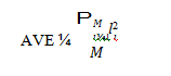
where li represents the loading of the lower-order component i of a specific higher-order construct measured with M lower-order components (i 5 1,… M). For this study, the AVE was 0.57828 (Appendix 3), which was clearly above the 0.5 threshold, therefore, indicating convergent validity for fin_risk (Sarstedt et al., 2017).
The composite reliability was defined as
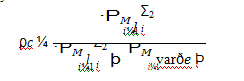
where ei is the measurement error of the lower-order component i, and var(ei) denotes the variance of the measurement error, which was defined as 1 l 2. Entering the two loading values yielded 0.788 (Appendix 3).
The statistics relevant for manually computing the higher-order construct’s HTMT values. The higher-order construct’s average heterotrait–heteromethod correlation with cperf was the average cross-loading of the cperf indicators with the mkt_risk, op_risk, and tech_risk constructs, which was 0.206, sperf was 0.192, fperf was 0.239 and reperf was 0.169 (Appendix 3).
In the next step, all monotrait–heteromethod correlations that were relevant for assessing the higher-order construct were computed. Since cperf was a ten-item construct, its average monotrait–heteromethod correlation was by definition 0.631. The eight items of sperf had item correlations, its average monotrait-heteromethod correlation was 0.586. Nineteen items of fperf had an average monotrait-heteromethod correlation of 0.576. The three items of reperf had an item correlation of 0.569 (Appendix 3).
The average monotrait–heteromethod correlation of the fin_risk construct was equal to the construct correlation among mkt_risk, op_risk, and tech_risk, which was 0.398. Finally, the quotient of the heterotrait–heteromethod correlations and the geometric mean of the average monotrait–heteromethod correlations was computed.
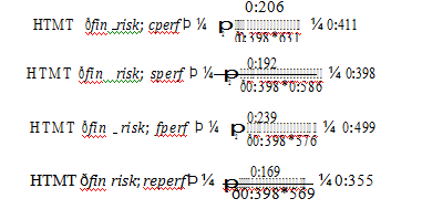
All values were lower than the conservative threshold of 0.85, thereby providing clear evidence for the higher-order construct’s reliability and validity. Furthermore, the structural model (Figure 1) was analyzed by using bootstrapping with 5,000 subsamples (no sign changes) and it was found that all structural model relationships were significant (p < 0.05; Table 7). The construct fin_risk had the strongest effect on fperf (0.422). The effect of fin_risk on reperf (0.321), fin_risk on sperf (0.227) and fin_risk on cperf (0.218) were, in comparison, notably smaller. The R2 values of all the dependent latent variables (i.e. cperf: 0.048, sperf: 0.052; fperf: 0.178; reperf: 0.103) were relatively low (Table 8).
The same holds for the blindfolding-based Q2 values, all of which were larger than zero (Table 8). Finally, f2 values were small independent variables cperf, sperf and reperf as compared to the moderate effect in fperf (Cohen, 1988) (see Table 9).
Model measurement for models 2, 3, 4 and 5
To ascertain the validity and reliability of the results, diagnostic tests were carried out as suggested by Hair et al. (2014a, b). The tests included internal consistency reliability (i.e. indicator and construct reliability tests) and construct validity were measured using convergent and discriminant validity. A multicollinearity test was conducted among the exogenous variables. The results were presented based on the study models. The paper followed the approach used in Wong (2019) and Hair Jr et al. (2017b, c) by conducting internal consistency reliability tests using the indicator and construct reliability tests respectively.
According to Wong (2019), indicator reliability is a rigorous tool for examining the unidimensionality of a set of scale items. This test was analyzed based on rho_A (ρ) result. The rho_A (ρ) provides a better measure of indicator reliability as compared to the use of Cronbach alpha (α) (Hair et al., 2014a, b; Henseler et al., 2016). Chin (2010) proposed that rho_A (ρ) scores should be > 0.70. Table 10 presented the results of models (2, 3, 4, and 5) indicator and construct reliability.

It could be deduced from Table 10 that the indicator reliability was achieved in all the models since the rho_A (ρ) scores of each of their respective constructs met the expected criteria. More precisely, the rho_A scores for the constructs in Model 2 ranged from 0.919 to 0.978. Also, the rho_A scores for the constructs in Model 3 ranged from 0.830 to 0.967; Model 4’s rho_A scores for its constructs ranged from 0.861 to 0.984 and finally, Model 5’s rho_A scores for its constructs ranged from 0.856 to 0.970. In terms of construct reliability which is relevant for assessing the extent to which a given construct is well measured by its indicators when combined, the result was obtained based on the composite reliability results (Bagozzi and Yi, 1988; Ringle et al., 2012). These scholars suggested composite reliability is met when its scores are ≥ 0.70; meeting this criterion implies that all the assigned indicators are relevant in analyzing a given construct.
From Table 10, all the various indicators in their associated models had strong mutual relationships with their respective constructs. In Model 2, for instance, the construct reliability scores of Model 2’s indicators ranged from 0.920 to 0.965; Model 3’s constructs had construct reliability ranging from 0.883 to 0.966; Model 4’s constructs had construct reliability ranging from 0.881 to 0.965 and finally, Model 5’s constructs had construct reliability ranging from 0.881 to 0.965. It could be deduced that all the indicators measuring each construct in all the models were relevant.
Convergent and discriminant validity
Following Hair et al. (2010, 2011), Rouibah et al. (2011), the test of convergent and discriminant validity was performed. Convergent validity considers the degree to which items measuring the same concept agree; discriminant measures the degree to which particular construct differs from the other constructs in the model (Hasan et al., 2012). Convergent validity relies on the AVE values of all the variables used in the SEM model. Fornell and Larcker (1981) recommended that a construct shows convergent validity if its AVE is less than 0.50. Thus, the AVE scores of each construct should be ≥ 0.50 to show that the measurement scale was convergent. The AVE scores of all the models’ constructs were presented in Table 11.
From Table 11, it could be seen that convergent validity was achieved in each of the study’s models. This is because all the AVEs met the criteria recommended by Fornell and Larcker (1981). Model 2, for instance, had AVE scores between 0.596 and 0.890; Model 3 had AVE scores between 0.597 and 0.719; Model 4 had AVE scores between 0.594 and 0.713 and finally, Model 5 had AVE scores between 0.557 and 0.901. These AVE scores in each model > 0.5 thus indicating convergent validity.
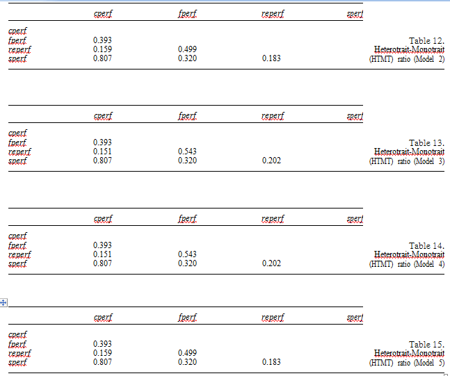
According to Hasan et al. (2012), discriminant validity explains how each construct is different from the others in the model. The test is to examine the cross-loadings of the indicators (Hair et al., 2011). Discriminant validity was reported using the Heterotrait- Monotrait (HTMT) ratio suggested by Sarstedt et al. (2014). According to Sarsdedt et al. (2014), HTMT ratio has the strength of detecting the absence of discriminant validity in common research scenarios as against the commonly used Fornell-Larcker criterion and cross-loadings criteria. The rule of thumb is that all HTMT values, which shows the correlation values among the latent variables, should be < 0.85 (Wetzels et al., 2009). The HTMT ratio for all the Models was reported in Tables 12–15.
From Tables 12–15, it could be deduced that all the values for each of the constructs in all the models were below HTMT.85. These indicate each construct under each model was distinct from the other.
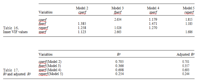
Test of Multicollinearity
The test of multicollinearity among the exogenous variables of the four models was checked using the inner variable inflation factor (VIF) values. According to Hair et al. (2014a, b), multicollinearity test is carried out to ensure that the study’s path coefficients are free from bias coupled with reducing the significant levels of collinearity among the predictor’s constructs. The rule of thumb is that VIF values should be < 5 to indicate the development of a good PLS-SEM model (Hair et al., 2014a, b). The results of the models’ inner VIF scores were presented in Table 16.
From Table 16, the inner values of the predictor’s constructs in Model 2 were less than the recommended value of 5; with the values ranging from 1.123 (sperf) and 1.385 (fperf). This indicated an absence of multicollinearity between the exogenous variables in Model 2. Also, in Model 3, the inner VIF values of the predictor’s constructs were 2.634 (cperf), 1.026 (reperf), and 2.663 (sperf) < 5 indicating the absence of multicollinearity between the Model’s exogenous variables. The inner VIF values of the predictor’s constructs in Model 4 were 1.179 (cperf), 1.471(fperf), and 1.270 (reperf) < 5 which indicated the absence of multicollinearity among the exogenous variables. Finally, the inner VIF values of the predictor’s constructs in Model 5 were 1.815 (cperf), 1.183 (fperf) and 1.686 (sperf) < 5. These inner VIF values clearly showed the absence of multicollinearity among the exogenous variables in the Models. The ensuing sections presented the results and discussion of the model’s results.
Test of structural model predictive accuracy
The coefficient of determination (R2 value) was used to compute the structural model’s predictive accuracy; calculated as the squared correlation between a specific endogenous construct’s actual and predicted values (Hair et al., 2014a, b). The R2 gives us the combined effect of independent variables on the dependent variable, i.e. it represents the amount of variance in the endogenous constructs explained by all of the exogenous constructs linked to it (Hair et al., 2014a, b). The R2 value of cperf (dependent variable) was 0.705, i.e. the combined effect of all the independent variables can cause a 70.5% variation in cperf (dependent variable) for Model 2. For Model 3, R2 value obtained for fperf was 36.6%. In Model 4 and 5, R2 values obtained for sperf (dependent variable) and reperf (dependent variable) were 69.8 and 25.4% respectively. Hence, one can conclude that the explanatory power of the model of this study was quite high (see Table 17).
According to Cohen (1988), f2 values of 0.02, 0.15, and 0.35, respectively represent small, medium, and large effect of the exogenous latent variable. It was observed the effect size of variables in Model 2 ranged from small effect (<0.15) to large effect (>0.35), in Model 3 effect size ranged from small (<0.15) to moderate (<0.35), in Model 4, the effect size was large (>0.35) and finally, in Model 5, the effect size was moderate (<0.35) (see Table 18).
While the R2 values denote predictive accuracy the predictive relevance Q2 indicates the model’s predictive relevance which is called Stone–Geisser’s Q2 value (Geisser, 1974; Stone, 1974). The Q2 values larger than zero for certain reflective endogenous latent variables indicate the path model’s predictive relevance for the construct (Hair et al., 2014a, b). The Q2 values were greater than zero as shown in Table 19 which indicates the path model’s predictive relevance was high.
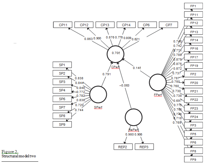
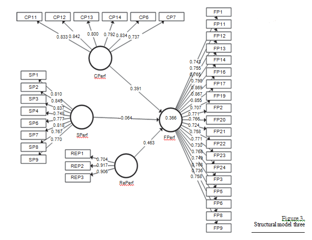
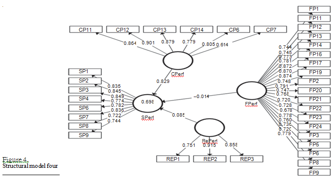
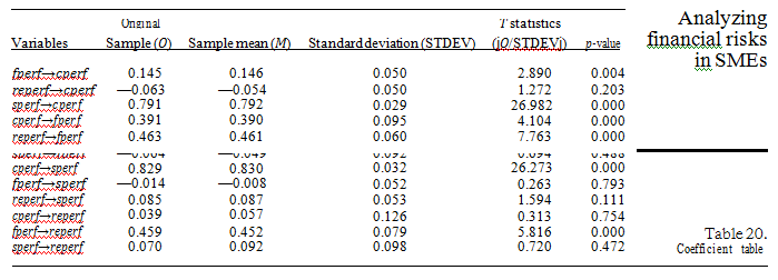
The research models proposes a total of 12 hypotheses for predicting the various dependent variables (cperf in Model 2 – Figure 2, fperf in Model 3 – Figure 3, sperf in Model 4 – Figure 4 and reperf in Model 5 – Figure 5), First three hypotheses were tested and two had direct relations from independent variables like fperf and sperf with cperf, i.e. the dependent variable. Running the PLS algorithm and bootstrapping calculations in SmartPLS software provided the path coefficient of these relations which denotes the strength of the relationships and p-value for verifying whether the relationship is statistically significant (see Table 20).
Furthermore, models 4 and 5 are shown in Figures 4 and 5 respectively.
It was found that fperf→cperf and sperf→cperf were statistically significant while reperf→cperf was not. The direct influence of fperf and sperf on the cperf for the study were significant. The influence of sperf had the maximum value (0.791), followed by fperf (0.145). The influence of reperf on cperf was not significant. With FPerf as the dependent variable (model 2), both cperf and reperf the relationship between the variables were statistically significant. The test of relationship resulted in 0.391 and 0.463 for cperf and reperf respectively. In model 4, the only cperf had a statistically significant relationship with SPerf (0.829). Model 5 had one statistically significant relationship. FPerf had an effect of 0.459 on reperf.
Results and Discussion
In model one, the objective was to analyze the effect of financial risks on the performance of the food processing firms in the selected cities. From the results, it was deduced that increased financial risks lead to increased financial performance. Financial risks cause firms to be more creative and innovative in their processes and procedures, hence leading to efficiency and ultimately increase financial performance. In periods of financial uncertainty, decision- makers try to explore all available options in order not to be wasteful. The resultant effect is that they tend to be prudent in the management of funds and ultimately improved upon their financial performance. Noor and Abdalla (2014) found financial risks impacts on financial performance. Christopoulos and Barratt (2016), Mentel et al. (2016), and Ol´ah et al. (2019) found financial risks impact on firm performance. Similarly, it was found that resource performance increases as financial risk increases. Financial risks compel firms to be cautious about resource utilization. Perceived financial risks oblige firms to employ strategies to cut down waste and employ operational processes that are efficient, productive, and profitable. O€zbug˘day et al. (2019) also concluded there is a positive and significant relationship between resource efficiency venture performances.
Higher financial risk could render a firm’s product and process obsolete and ultimately make it uncompetitive. Accordingly, firms respond to such situations with increasing social and corporate responsibilities. This enables them to maintain their reputation and social support. The aim is to win favor from their communities or markets. Boutin-Dufresne and Savaria (2004) concluded that CSR contributes positively to a firm’s long-term risk-adjusted- performance. K€olbel et al. (2017) found that corporate social irresponsibility creates a financial risk for a business. Meanwhile, it was observed that increased financial risks lead to increased compliance with regulations. The sector is heavily regulated and firms are expected to comply with all operational requirements. Failure to comply with regulations could result in sanctions by the regulator, which could compound the financial risk exposure of the business.
Therefore, owners/managers would be extra careful not to attract any sanction or negative publicity by the regulators in times of rising financial risks. This could lead to a reduction in customer share, sales, profitability, and bring about competitive disadvantage. As O€zbug˘day et al. (2019) submit, compliance through resource efficiency strategy could boost sales.
Next, models 2, 3, 4 and 5 sought to analyze the relationship between the performance variables. From model 2, it was observed fperf and sperf significantly influenced cperf. This implies that as SMEs in the food industry gain better financial standing, they can comply with various rules and regulations that concern the environment and their work operations. Also, as SMEs in the industry seek the welfare of their employees, customers, and the community in which they operate, it improves their compliance performance as well. Furthermore, in Model 3, it was found that cperf and reperf had a statistically significant relationship with fperf. These relationships were both positive as well. The results suggest that as SMEs in the industry comply with rules and regulations concerning the environment, labor issues and others, they gain better financial standing such as an increase in product value, higher return on investment, an increase in market share and many more. Moreover, as SMEs use their resources efficiently through re-use and recycling materials, they gain better financial standing (O€zbug˘day et al., 2019).
The results indicate cperf had a statistically significant positive effect on sperf. This means the more an SME complies with laws, their social performance significantly improves.

Finally, model 5 also depicts a statistically significant relationship between fperf and reperf. This suggests that an SME with good financial performance can influence its resource use efficiency. This is because reusing and recycling of materials require the right investment into the right machinery. Therefore, Liu (2020) concluded a business must have sufficient financial resources to enable them to implement efficient environmental programs.
Implications of the study Practical implication – Firms in the food processing sector must identify and manage financial risks as they positively influence their operations. They should proactively acquire and deploy technologies that make them competitive in terms of resource use, social acceptance, and financial capability. Managers need to comply with regulations and deploy the necessary tools and techniques to operate in a resource-efficient manner since these practices have a positive relationship with financial risks. Due to the heavy regulations in the food processing sector, firms need to avoid sanctions that would ruin their reputation. It is, therefore, necessary owners/managers adopt the appropriate business strategies to reduce their risks.
- Policy implication – The study revealed that financial risk was the one single variable that plays a significant role in food processing. This implies that policy initiatives and interventions that tend to minimize the elements in the SMEs’ operations that tend to increase their financial risk exposure including the procedure and cost of credit, access and cost of technology and the various regulations (e.g. taxation). Policy initiatives including tax breaks, interest rate ceiling and subsidies for SMEs could promote their activities. Besides, the firm’s internal policy should aim at reducing the risk exposure in their engagement with stakeholders (customers, creditors, suppliers etc.). Implementing credit policy in the business is an example of such policies. Furthermore, policy interventions should include business development services that expose food processors to different financial risks – how to identify, assess and manage these risks.
- Theoretical implication – The stakeholder theory highlights the business–stakeholder interactions in the environment, focusing on the interest and power the different actors within the business space. The study points out and suggests the need to highlight the financial risks exposure of businesses as a result of the interactions. Therefore, the idea of financial risks posed by these actors as the businesses engage them should be of theoretical significance to researchers. The paper contributes to the information asymmetry theory. The findings of the study show that the issue of risks due to non-disclosure of relevant information (information asymmetry) could emanate from any of the actors in the value chain and not only from the SMEs at it has often been interpreted. For instance, both the Financial Institution and SME could contribute to the financial risk exposure of either party due to non-disclosure of relevant information resulting in adverse selection.
- Implications for future research – Future research should look at extending such as analysis into other sectors including larger firms in the sector and other sectors. An issue that would be interesting investigating would be the effect of firm characteristics or even sectorial differences in predicting the financial risk–firm performance relationship.
References
Abdallah, Z.M., Md AMIN, M.A., Sanusi, N.A. and Kusairi, S. (2014), “Impact of size and ownership structure on efficiency of Commercial Banks in Tanzania: stochastic Frontier analysis”, International Journal of Economic Perspectives, Vol. 8 No. 4, pp. 66-76.
Abeyrathna, G.M. and Kalainathan, K. (2016), “Financial risk, financial risk management practices and performance of Sri Lankan SMEs: special reference to Anuradhapura district”, Research Journal of Finance and Accounting, Vol. 15 No. 7, pp. 16-22.
Abimbola, O.A. and Kolawole, O.A. (2017), “Effect of working capital management practices on the performance of small and medium enterprises in Oyo state, Nigeria”, Asian Journal of Economics, Business and Accounting, Vol. 3 No. 4, pp. 1-8.
Agyapong, D. and Attram, A.B. (2019), “Effect of owner-managers financial literacy on the performance of SMEs in the Cape Coast Metropolis in Ghana”, Journal of Global Entrepreneurship Research, Vol. 9 No. 1, pp. 1-13.
Al-Khouri, R. (2011), “Assessing the risk and performance of the GCC banking sector”, International Research Journal of Finance and Economics, Vol. 65 No. 1, pp. 72-81.
Asgary, A., Ozdemir, A.I. and O€zyu€rek, H. (2020), “Small and medium enterprises and global risks: evidence from manufacturing SMEs in Turkey”, International Journal of Disaster Risk Science, Vol. 11 No. 1, pp. 59-73.
Babin, B.J., Hair, J.F. and Boles, J.S. (2008), “Publishing research in marketing journals using structural equation modelling”, Journal of Marketing Theory and Practice, Vol. 16 No. 4, pp. 279-286.
Bagozzi, R.P. and Fornell, C. (1982), “Theoretical concepts, measurements, and meaning”, A Second Generation of Multivariate Analysis, Vol. 2 No. 2, pp. 5-23.
Bagozzi, R.P. and Yi, Y. (1988), “On the evaluation of structural equation models”, Journal of the Academy of Marketing Science, Vol. 16 No. 1, pp. 74-94.
Bartlett, J.E., Kotrlik, J.W. and Higgins, C.C. (2001), “Organizational research: determining the appropriate sample size in survey research”, Information Technology, Learning, and Performance Journal, Vol. 19 No. 1, pp. 43-50.
Bbenkele, E.K. (2007), “An investigation of Small and Medium Enterprises perceptions towards services offered by Commercial banks in South Africa”, African Journal of Accounting, Economics, Finance and Banking Research, Vol. 1 No. 1, pp. 12-25.
Belas, J., Smrcka, L., Gavurova, B. and Dvorsky, J. (2018), “The impact of social and economic factors in the credit risk management of SME”, Technological and Economic Development of Economy, Vol. 24 No. 3, pp. 1215-1230.
Bet´akov´a, J., Lorko, M. and Dvorsky´, J. (2014), “The impact of the potential risks of the implementation of instruments for environmental area management on the development of urban settlement”, WIT Transactions on Ecology and the Environment, Vol. 181, pp. 91-101.
Boermans, M.A. and Willebrands, D. (2011), Firm Performance under Financial Constraints and Risks: Recent Evidence from Microfinance Clients in Tanzania, HU University of Applied Sciences Utrecht, Utecht.
Boutin-Dufresne, F. and Savaria, P. (2004), “Corporate social responsibility and financial risk”, Journal of Investing, Vol. 13 No. 1, pp. 57-66.
Cabedo, J.D. and Tirado, J.M. (2004), “The disclosure of risk in financial statements”, June, Accounting Forum, Vol. 28 No. 2, pp. 181-200.
Chin, W.W. (2010), “How to write up and report PLS analyses”, Handbook of Partial Least Squares, Springer, Berlin, Heidelberg, pp. 655-690.
Christopoulos, A.D. and Barratt, J.G. (2016), “Credit risk findings for commercial real estate loans using the reduced form”, Finance Research Letters, Vol. 19, pp. 228-234.
Cipovov´a, E. and Dlaskov´a, G. (2016), “Comparison of different methods of credit risk management of the Commercial bank to accelerate lending activities for SME segment”, European Research Studies Journal, Vol. 19 No. 4, pp. 17-26.
Civelek, M. (2018), Essentials of Structural Equation Modeling, Istanbul Ticaret University, Zea Books, The University of Nebraska, doi: 10.13014/K2SJ1HR5.
Cohen, J. (1988), Statistical Power Analysis for the Behavioral Sciences, 2nd ed., Erlbaum, Hillsdale, NJ.
Deng, X.X. (2020), “Empirical analysis of financial risks of Corporate M and A based on big data”, January, 2019 3rd International Conference on Education, Economics and Management Research, pp. 454-457.
Dimitropoulos, P.E., Asteriou, D. and Koumanakos, E. (2010), “The relevance of earnings and cash flows in a heavily regulated industry: evidence from the Greek banking sector”, Advances in Accounting, Vol. 26 No. 2, pp. 290-303.
Ekaterina, S. and Thielmann, K. (2020), “Financial Risks and Management”, International Encyclopedia of Human Geography, 2nd ed., Elsevier, pp. 139-145.
Eniola, A.A. and Entebang, H. (2015), “SME firm performance-financial innovation and challenges”,
Procedia-Social and Behavioral Sciences, Vol. 195, pp. 334-342.
Fornell, C. and Larcker, D.F. (1981), “Structural equation models with unobservable variables and measurement error: algebra and statistics”, Journal of Marketing Research, Vol. 18 No. 3, pp. 382-388.
Franke, G. and Sarstedt, M. (2019), “Heuristics versus statistics in discriminant validity testing: a comparison of four procedures”, Internet Research, Vol. 29 No. 3, pp. 430-447.
Freeman, R.E., Harrison, J.S., Wicks, A.C., Parmar, B.L. and De Colle, S. (2010), Stakeholder Theory: The State of the Art, Cambridge University Press, Cambridge.
Freeman, R.E. (1984), Strategic Management: A Stakeholder Approach, Pitman Publishing, Boston. Gabriel, S.C. and Baker, C.B. (1980), “Concepts of business and financial risk”, American Journal of
Agricultural Economics, Vol. 62 No. 3, pp. 560-564.
Gefen, D. and Straub, D.W. (2000), Managing User Trust in B2C e-services Quarterly, Electronic Publication.
Geisser, S. (1974), “A predictive approach to the random effect model”, Biometrika, Vol. 61 No. 1, pp. 101-107.
Gou, Q. and Huang, Y. (2019), Financing support schemes for SMEs in China: benefits, costs and selected policy issues, The Chinese Economic Transformation, p. 193.
Hacievliyagil, N. and Eksi, I_.H. (2019), “A micro-based study for bank credit and economic growth: manufacturing sub-sectors analysis”, South East European Journal of Economics and Business, Vol. 14 No. 1, pp. 72-91.
Hair, J.F., Black, W.C., Babin, B.J., Anderson, R.E. and Tatham, R.L. (2006), “SEM: confirmatory factor analysis”, Multivariate Data Analysis, Pearson Prentice Hall, Upper Saddle River, pp. 770-842.
Hair, J.F., Black, W.C., Babin, B.J. and Anderson, R.E. (2010), Confirmatory Factor Analysis, Multivariate Data Analysis, 7th ed., Upper Saddle River, NJ, USA, pp. 600-638.
Hair, J.F., Ringle, C.M. and Sarstedt, M. (2011), “PLS-SEM: indeed a silver bullet”, Journal of Marketing Theory and Practice, Vol. 19 No. 2, pp. 139-151.
Hair, J.F., Sarstedt, M., Hopkins, L. and Kuppelwieser, V.G. (2014a), “Partial least squares structural equation modeling (PLS-SEM)”, European Business Review, Vol. 26 No. 2, pp. 106-121.
Hair, J.F., Hult, G.T.M., Ringle, C.M. and Sarstedt, M. (2014b), A Primer on Partial Least Squares Structural Equation Modeling (PLS-SEM), SAGE, Los Angeles.
Hair, J.F., Babin, B.J. and Krey, N. (2017a), “Covariance-based structural equation modeling in the journal of advertising: review and recommendations”, Journal of Advertising, Vol. 46 No. 1, pp. 163-177.
Hair, J.F., Matthews, L.M., Matthews, R.L. and Sarstedt, M. (2017b), “PLS-SEM or CB-SEM: updated guidelines on which method to use”, International Journal of Multivariate Data Analysis, Vol. 1 No. 2, pp. 107-123.
Hair, J.F., Sarstedt, M., Ringle, C.M. and Gudergan, S.P. (2017c), Advanced Issues in Partial Least Squares Structural Equation Modelling, SAGE publications, New York.
Haniff, B.A., Akma, L., Lee, S. and Finance, D. (2017), Access to Financing for SMEs: Perception and Reality, Bank Negara Malaysia, pp. 1-6.
Hasan, L., Morris, A. and Probets, S. (2012), “A comparison of usability evaluation methods for evaluating e-commerce websites”, Behaviour and Information Technology, Vol. 31 No. 7, pp. 707-737.
Henri, J.F. (2006), “Organizational culture and performance measurement systems”, Accounting, Organizations and Society, Vol. 31 No. 1, pp. 77-103.
Henseler, J., Ringle, C.M. and Sarstedt, M. (2015), “A new criterion for assessing discriminant validity in variance-based structural equation modelling”, Journal of the Academy of Marketing Science, Vol. 43 No. 1, pp. 115-135, doi: 10.1007/s11747-014-0403-8.
Henseler, J., Hubona, G. and Ray, P.A. (2016), “Using PLS path modeling in new technology research: updated guidelines”, Industrial Management and Data Systems, Vol. 116 No. 1, pp. 2-20.
Huhtilainen, M. (2020), “The determinants of bank insolvency risk: evidence from Finland”, Journal of Financial Regulation and Compliance, Vol. 28 No. 2, pp. 315-335.
Hulland, J. (1999), “Use of partial least squares (PLS) in strategic management research: a review of four recent studies”, Strategic Management Journal, Vol. 20 No. 2, pp. 195-204.
Ilyas, S. (2019), “Banks’ lending preferences and SME credit in Pakistan: experience and way forward”, International Journal of Advanced Economics, Vol. 1 No. 1, pp. 134-142.
Jayaratne, J. and Strahan, P.E. (1996), “The finance-growth nexus: evidence from bank branch deregulation”, Quarterly Journal of Economics, Vol. 111 No. 3, pp. 639-670.
Jenkins, H. (2004), “A critique of conventional CSR theory: an SME perspective”, Journal of General Management, Vol. 29 No. 4, pp. 37-57.
Jones, P., Maas, G., Dobson, S., Newbery, R., Agyapong, D. and Matlay, H. (2018), “Entrepreneurship in Africa, Part 3: conclusions on African entrepreneurship”, Journal of Small Business and Enterprise Development, Vol. 25 No. 5, pp. 706-709.
Jones, T.M. (1995), “Instrumental stakeholder theory: a synthesis of ethics and economics”, Academy of Management Review, Vol. 20, pp. 404-437.
Jorge, M.J.D.S. and Augusto, M.A.G. (2011), “Financial risk exposures and risk management: evidence from European nonfinancial firms”, Revista de Administraç~ao Mackenzie, Vol. 12 No. 5, pp. 65-97.
Joshi, A., Kale, S., Chandel, S. and Pal, D.K. (2015), “Likert scale: explored and explained”, British Journal of Applied Science and Technology, Vol. 7 No. 4, p. 396.
Khan, B. (2020), “Microfinance banks and its impacts on small and medium scale enterprises in Nigeria”, World Scientific News, Vol. 141, pp. 115-131.
K€olbel, J.F., Busch, T. and Jancso, L.M. (2017), “How media coverage of corporate social irresponsibility increases financial risk”, Strategic Management Journal, Vol. 38 No. 11, pp. 2266-2284.
Kozak, L.S. and Danchuk, M.V. (2016), “Evolution of enterprise risk management under current conditions of economic development: from fragmented to integrated”, Aкmyaльн{ nроблемu економ{кu, No. 4, pp. 23-29.
Kundid, A. and Ercegovac, R. (2011), “Credit rationing in financial distress: Croatia SMEs’ finance approach”, International Journal of Law and Management, Vol. 53 No. 1, pp. 62-84.
Latan, H. and Noonan, R. (Eds) (2017), Partial Least Squares Path Modeling: Basic Concepts, Methodological Issues and Applications, Springer, Berlin.
Lindsey, T. and Butt, S. (2020), “Indonesian financial laws: banking, insolvency and taxation”, in
Research Handbook on Asian Financial Law, Edward Elgar Publishing.
Liu, Z. (2020), “Unraveling the complex relationship between environmental and financial performance- a multilevel longitudinal analysis”, International Journal of Production Economics, Vol. 219, pp. 328-340.
Mentel, G., Szetela, B. and Tvaronaviciene, M. (2016), “Qualifications of Managers vs. Effectiveness of investment funds in Poland”, Economics and Sociology, Vol. 9, pp. 126-136.
Morgan, L., Chisoro, C. and Karodia, A.M. (2015), “An evaluation of the impact of organisational culture on employee work performance: a case study of a FET College in Durban”, Oman Chapter of Arabian Journal of Business and Management Review, Vol. 34 No. 2614, pp. 1-44.
Motta, V. and Sharma, A. (2019), “Lending technologies and access to finance for SMEs in the hospitality industry”, International Journal of Hospitality Management, Vol. 86, p. 102371.
Moyi, E. (2019), “Riskiness of lending to small businesses: a dynamic panel data analysis”, The Journal of Risk Finance, Vol. 20 No. 1, pp. 94-110.
Nasiri, M., Ukko, J., Saunila, M., Rantala, T. and Rantanen, H. (2020), “Digital-related capabilities and financial performance: the mediating effect of performance measurement systems”, Technology Analysis and Strategic Management, pp. 1-14.
Neacs¸u, M.C., Negut¸, S. and Vl˘asceanu, G. (2018), “The impact of geopolitical risks on tourism”,
Amfiteatru Economic, Vol. 20 No. 12, pp. 870-884.
Nguyen, T.V., Ngoc, T.B.L.E. and Freeman, N.J. (2006), “Trust and uncertainty: a study of bank lending to private SMEs in Vietnam”, Asia Pacific Business Review, Vol. 12 No. 4, pp. 547-568.
Noor, J.A.M. and Abdalla, A.I. (2014), “The impact of financial risks on the firms’ performance”,
European Journal of Business and Management, Vol. 6 No. 5, pp. 97-101.
Nyquist, H. (2002), “Certain topics in telegraph transmission theory”, Proceedings of the IEEE, Vol. 90 No. 2, pp. 280-305.
Offiong, A., Udoka, C.O. and Bassey, J.G. (2019), “Financial risk and performance of small and medium enterprises in Nigeria”, Investment Management and Financial Innovations, Vol. 16 No. 4, pp. 54-67.
Ol´ah, J., Kov´acs, S., Virglerova, Z., Lakner, Z., Kovacova, M. and Popp, J. (2019), “Analysis and comparison of economic and financial risk sources in SMEs of the Visegrad group and Serbia”, Sustainability, Vol. 11 No. 7, p. 1853.
Ombworo, E.O. (2014), “The Effect of Liquidity on the Profitability of Small and Medium-Size Enterprises in Kenya”, Unpublished MBA Project, University of Nairobi, Nairobi.
Owusu, E.B. (2019), “Financing challenges faced by SMEs in Ghana”, working paper, Oulu Business School, Oulu.
O€zbug˘day, F.C., Findik, D., O€zcan, K.M. and Bas¸çi, S. (2019), “Resource efficiency investments and firm performance: evidence from European SMEs”, Journal of Cleaner Production, Vol. 252, p. 119824.
Pallant, J. (2011), Survival manual, A step by step guide to data analysis using SPSS.
Polites, G.L., Roberts, N. and Thatcher, J. (2012), “Conceptualizing models using multidimensional constructs: a review and guidelines for their use”, European Journal of Information Systems, Vol. 21 No. 1, pp. 22-48.
Qin, X. and Pastory, D. (2012), “Comparative analysis of commercial banks liquidity position”, The Case of Tanzania, Vol. 7 No. 10, pp. 134-141.
Rao, P., Kumar, S., Gaur, V. and Verma, D. (2017), “What constitutes financing gap in Indian SMEs–owners’ perspective?”, Qualitative Research in Financial Markets, Vol. 9 No. 2, pp. 117-131.
Regasa, D., Fielding, D. and Roberts, H. (2019), “Sources of financing and firm growth: evidence from Ethiopia”, Journal of African Economies, Vol. 29 No. 1, pp. 26-45.
Ringle, C.M., Sarstedt, M. and Straub, D.W. (2012), “Editor’s comments: a critical look at the use of PLS-SEM in, ‘MIS Quarterly’”, MIS Quarterly, pp. iii-xiv.
R€onkk€o, M. and Evermann, J. (2013), “A critical examination of common beliefs about partial least squares path modelling”, Organizational Research Methods, Vol. 16 No. 3, pp. 425-448.
Rouibah, K., Ramayah, T. and May, O.S. (2011), “Modeling user acceptance of internet banking in Malaysia: a partial least square (PLS) approach”, in E-adoption and Socio-Economic Impacts: Emerging Infrastructural Effects, IGI Global, pp. 1-23.
Ruziqa, A. (2013), “The impact of credit and liquidity risk on bank financial performance: the case of Indonesian Conventional Bank with total asset above 10 trillion Rupiah”, International Journal of Economic Policy in Emerging Economies, Vol. 6 No. 2, pp. 93-106.
Sarstedt, M., Ringle, C.M., Smith, D., Reams, R. and Hair, J.F. Jr (2014), “Partial least squares structural equation modelling (PLS-SEM): a useful tool for family business researchers”, Journal of Family Business Strategy, Vol. 5 No. 1, pp. 105-115.
Sarstedt, M., Ringle, C.M. and Hair, J.F. (2017), “Partial least squares structural equation modelling”,
Handbook of Market Research, Vol. 26, pp. 1-40.
Schumpeter, J. (1911), The theory of economic development, Harvard Economic Studies, New York. Sekaran, U. and Bougie, R. (2003), Research Methods for Business: A Skill Building Approach, John
Willey & Sons, New York.
Selvam, M., Gayathri, J., Vasanth, V., Lingaraja, K. and Marxiaoli, S. (2016), “Determinants of firm performance: a subjective model”, International Journal of SocialScience Studies, Vol. 4, p. 90.
Shaverdi, M., Yaghoubi, S. and Ensafian, H. (2020), “A multi-objective robust possibilistic model for technology portfolio optimization considering social impact and different types of financing”, Applied Software Computing, Vol. 86, p. 105892.
Stone, M. (1974), “Cross-validatory choice and assessment of statistical predictions (with Discussion)”,
Journal of the Royal Statistical Society: Series B, Vol. 36 No. 11, pp. 1-147.
Tafri, F.H., Hamid, Z., Meera, A.K.M. and Omar, M.A. (2009), “The impact of financial risks on the profitability of Malaysian commercial banks: 1996-2005”, International Journal of Social, Human Science and Engineering, Vol. 3 No. 6, pp. 268-282.
Utomo, M.N., Cahyaningrum, W. and Kaujan, K. (2020), “The role of entrepreneur characteristic and financial literacy in developing business success”, Jurnal Manajemen Bisnis, Vol. 11 No. 1, pp. 26-42.
Van Greuning, H. and Brajovic Bratanovic, S. (2009), Analyzing Banking Risk a Framework for Assessing Corporate Governance and Financial Risk, The World Bank, Geneva.
Voorhees, C.M., Brady, M.K., Calantone, R. and Ramirez, E. (2016), “Discriminant validity testing in marketing: an analysis, causes for concern, and proposed remedies”, Journal of the Academy of Marketing Science, Vol. 44 No. 1, pp. 119-134.
Walsh, J.P. (2005), “Taking stock of stakeholder management”, Academy of Management Review, Vol. 30 No. 2, pp. 426-438.
Wasiuzzaman, S., Nurdin, N., Abdullah, A.H. and Vinayan, G. (2020), “Creditworthiness and access to finance of SMEs in Malaysia: do linkages with large firms matter?”, Journal of Small Business and Enterprise Development, Vol. 2 No. 27, pp. 197-217, doi: 10.1108/JSBED-03-2019-0075.
Wetzels, M., Odekerken-Schr€oder, G. and Van Oppen, C. (2009), “Using PLS path modeling for assessing hierarchical construct models: guidelines and empirical illustration”, MIS Quarterly, pp. 177-195.
Willits, F.K., Theodori, G.L. and Luloff, A.E. (2016), “Another look at Likert scales”, Journal of Rural Social Sciences, Vol. 31 No. 3, p. 6.
Wong, J.S. (2019), Fifth Chinese Daughter, University of Washington Press, Brooklyn, NE.
Xu, J. and Li, J. (2019), The impact of intellectual capital on SMEs’ performance in China, Journal of Intellectual Capital.
Yang, S., Zhang, Z., Zhou, J., Wang, Y., Sun, W., Zhong, X., Fang, Y., Yu, Q. and Qi, Y. (2020), “Financial risk analysis for SMEs with graph-based supply chain mining”, Proceedings of the Twenty-Ninth International Joint Conference on Artificial Intelligence, pp. 4661-4667.
Yang, B. (2020), “Construction of logistics financial security risk ontology model based on risk association and machine learning”, Safety Science, Vol. 123, p. 104437.
Yen, T.T.B., Le, B.M. and Tran, T.H. (2019), “Analysing the barriers to innovation development in emerging economies: Vietnamese Small and Medium Enterprises (SMEs) as an empirical case”, Asian Economic and Financial Review, Vol. 9 No. 1, p. 64.
Yiannaki, S.M. (2012), “A systemic risk management model for SMEs under financial crisis”,
International Journal of Organisational Analysis, Vol. 20 No. 4, pp. 406-422.
Yusuf, T.O. and Dansu, F.S. (2013), “SMEs, business risks and sustainability in Nigeria”, European Journal of Business and Social Sciences, Vol. 2 No. 9, pp. 76-94.
Further reading
Kumar, R. (2017), Targeted SME Financing and Employment Effects: What Do We Know and what Can We Do Differently?, World Bank, Geneva.
Laitinen, E.K. (2011), “Effect of reorganization actions on the financial performance of small entrepreneurial distressed firms”, Journal of Accounting and Organizational Change, Vol. 7 No. 1, pp. 57-95.
Also Read:- FI 300 Corporate Finance Assignment Answers
Appendix 1
| MR | MR | OR | MR | MR | TR | |
|
|
The firm is affected by changes in or misunderstanding of existing laws and policies related to the business | 0.851 | ||||
| Non-compliance with internal policies, procedures and best | 0.847 | |||||
| practices affect the firm | ||||||
| Loss of good reputation due to malpractices disrupts the | 0.790 | |||||
| firm’s operations | ||||||
| The firm is exposed to perceived fraud arising from assets | 0.650 | |||||
| embezzlement, manipulating financial statements, | ||||||
| corruption and bribery | ||||||
| The firm incurs cost whenever its people (employee) a 0.756 | ||||||
| breakdown or suffers damages | ||||||
| Defaults or delays in payment of debts by debtors disrupt 0.671 | ||||||
| the firm’s cash flow | ||||||
| The firm suffer losses whenever its partners fail to meet 0.691 | ||||||
| contractual obligations | ||||||
| The firm is threatened by any single or a group exposure | 0.538 | |||||
| with the potential to produce a large number of losses | ||||||
| The firm is exposed to recovery risk whenever it fails to | 0.531 | |||||
| quickly recover from credit defaults | ||||||
| The firm is exposed to credit detection risk whenever it fails | 0.488 | |||||
| to detect or accurately identify all credit defaulters | ||||||
| The firm activities are affected by changes, fluctuations or | 0.677 | |||||
| unpredictable nature of interest rates | ||||||
| Changes in the price of the currency to another affect the firm | 0.714 | |||||
| The firm is exposed to commodity risk due to frequent 0.772 | ||||||
| changes in prices and availability of commodities (raw | ||||||
| materials, end product) | ||||||
| The firm is exposed to monetary policy risk whenever the | 0.737 | |||||
| central bank makes changes in current monetary policies | ||||||
| The firm is exposed to market risk as a result of declines in 0.702 | ||||||
| the economic performance of the economy | ||||||
| Losses arising from the firm’s inability to sell its assets at | 0.793 | |||||
| the required value disrupt its operations | ||||||
| The firm faces funding liquidity risk due to our inability to | 0.781 | |||||
| settle bills or meet other short-term financial requirements | ||||||
| The need to regularly meet unplanned capital expenditure | 0.759 | |||||
| affects the firm’s operations | ||||||
| The firm is exposed to seasonal fluctuations in revenue | 0.731 | |||||
| generation | ||||||
| Continuous rise in interest rates make it difficult for the firm | 0.575 | |||||
| to take advantage of better financing options | ||||||
| The firm makes losses arising from damages to operating | 0.719 | |||||
| systems | ||||||
| The cost associated with acquiring technological | 0.827 | |||||
| infrastructure affects the firm’s operations | ||||||
| Exposure to cyberattacks or data breaches disrupts the | 0.900 | |||||
| firm’s operations | ||||||
| Telecommunicationandconnectivityissuesisarisk to the firm | 0.796 | |||||
| Table A1. Rotated component matrix | The firm faces data integrity risk because the data it stores
and processes are mostly incomplete, inaccurate and or inconsistent |
0.832 |
| CP | FP | FP | SP | FP | REP | SP | FP | ||
| We have experienced increasing economic | 0.792 | ||||||||
| value added | |||||||||
| Our return on equity has been improving | 0.855 | ||||||||
| Firm’s net income/revenue is increasing | 0.868 | ||||||||
| steadily | |||||||||
| Return on investment helps maintain our | 0.761 | ||||||||
| investors | |||||||||
| We have experienced increasing EBIT | 0.816 | ||||||||
| Margin | |||||||||
| The firm’s management is efficient at | 0.729 | ||||||||
| using its assets to generate earnings | |||||||||
| The firm can allocate a portion of its profit | 0.440 | ||||||||
| to owners | |||||||||
| The firm experienced appreciation in its | 0.653 | ||||||||
| worth | |||||||||
| We are getting more cashback for each | 0.677 | ||||||||
| cedi invested | |||||||||
| Market fluctuations have been favorable to | 0.565 | ||||||||
| our firm | |||||||||
| The firm is experiencing increasing | 0.609 | ||||||||
| product value | |||||||||
| The firm is earning a rate higher than its | 0.585 | ||||||||
| replacement cost | |||||||||
| The firm is experiencing a rising market- | 0.558 | ||||||||
| share growth | |||||||||
| Our firm has experienced asset growth | 0.641 | ||||||||
| over time | |||||||||
| We are experiencing net revenue growth | |||||||||
| There is net income growth appreciation | 0.593 | ||||||||
| The number of our employees is growing | 0.576 | ||||||||
| There is a relatively lower turnover rate in | 0.454 | ||||||||
| our firm | |||||||||
| We invest in employee’s development and | 0.451 | ||||||||
| training | |||||||||
| We have favorable wages and rewards | 0.556 | ||||||||
| policies | |||||||||
| The firm has career plans in place | 0.545 | ||||||||
| We have good organizational climate | 0.745 | ||||||||
| Our employees are generally satisfied | 0.759 | ||||||||
| Our customers are satisfied with our mix of | 0.775 | ||||||||
| products /services | |||||||||
| We receive less number of complaints | 0.758 | ||||||||
| Our products have high repurchase rate | 0.757 | ||||||||
| We have high new customer retention | 0.805 | ||||||||
| There is general customers satisfaction | 0.841 | ||||||||
| There are many new products/services | 0.610 | ||||||||
| launched | |||||||||
| We have projects to improve/recover the | 0.628 | ||||||||
| environment | Table A2.
Rotated component |
Appendix 2
| CP | FP | FP | SP | FP | REP | SP | FP | ||
| The firm has a low level of energy intensity | 0.541 | ||||||||
| (lower cost to convert energy) | |||||||||
| We use recyclable materials | 0.733 | ||||||||
| We reuse our residuals | 0.703 | ||||||||
| We monitor the volume of energy | 0.634 | ||||||||
| consumption | |||||||||
| The firm has not experienced any lawsuits | 0.553 | ||||||||
| due to its practices | |||||||||
| We have designed and follow our 0.856 | |||||||||
| environmental policy | |||||||||
| The firm produces an annual 0.879 | |||||||||
| environmental audit report | |||||||||
| There is an environmental review 0.863 | |||||||||
| committee | |||||||||
| We work to meet the international 0.711 | |||||||||
| environmental standard | |||||||||
| We have the local certifications and 0.596 | |||||||||
| operate within them | |||||||||
| We publish our annual environmental 0.849 | |||||||||
| audit report | |||||||||
| Our Board Size is comparable to that of 0.806 | |||||||||
| similar firms | |||||||||
| Our Board is free from any form of 0.825 | |||||||||
| interference | |||||||||
| We have directors who monitor executives 0.745 | |||||||||
| to act in the interest of shareholders | |||||||||
| Managers have high share ownership | 0.487 | ||||||||
| There is equity in terms of the number of 0.792 | |||||||||
| women and men in the firm | |||||||||
| We publish our reports periodically 0.822 | |||||||||
| We employ more people from minority 0.620 | |||||||||
| groups | |||||||||
| We have several social and cultural 0.660 | |||||||||
| projects | |||||||||
| Our firm has not experienced any lawsuits | 0.481 | ||||||||
| We meet regulatory agencies requirement | 0.733 | ||||||||
| We engage in fair trade | 0.837 | ||||||||
| We work to reduce vulnerability in our | 0.748 | ||||||||
| community | |||||||||
Table A2.
Note(s): Extraction Method: Principal Component Analysis Rotation Method: Varimax with Kaiser Normalization a Rotation converged in 10 iterations
¼ ð0:8686 þ 0:7293 þ 0:1369Þ=3AVE ¼ 0:9382 þ 0:8542 þ 0:3702 =3
¼ 1:7348=3
¼ 0:57828
ρC ¼ .0:938 þ 0:854 þ 0:370Þ2=ð0:938 þ 0:854 þ 0:370Σ2 þ .1 — 0:9382Σ
¼ 4:6742=4:6742 þ 0:1202 þ 0:2707 þ 0:8631
¼ 4:6742=5:92814
¼ 0:788
Average heterotrait-heteromethod correlation with cperf was the average cross loading of the cperf
indicators with the mkt_risk, op_risk and tech_risk constructs (Table 15), which was:
¼ð — 0:023 þ —0:004 þ 0:001 þ 0:045 þ 0:031 þ 0:176 þ —0:064 þ 0:019 þ —0:015 þ 0:102 þ 0:119 þ 0:197 þ 0:484 þ 0:632 þ 0:568 þ 0:376 þ 0:629 þ 0:429Þ=18
¼ 3:702=18
¼ 0:206
In the case of sperf, the same statistic was given by the average cross loadings of sperf indicators with mkt_risk, op_risk and tech_risk (Table 15), which was:
¼ð — 0:081 þ 0:136 þ —0:006 þ 0:047 þ 0:016 þ 0:036 þ 0:224 þ —0:025 þ —0:022
þ 0:111 þ 0:026 þ —0:047 þ 0:101 þ 0:038 þ 0:219 þ 0:087 þ 0:530 þ 0:432 þ 0:401 þ 0:326 þ 0:444 þ 0:552 þ 0:479 þ 0:582Þ=24
¼ 4:606=24
¼ 0:192
Fperf, the same statistic was given by the average cross loadings of Fperf indicators with mkt_risk, op_risk and tech_risk (Table 15), which was:
¼ ð0:222 þ 0:260 þ 0:217 þ 0:346 þ 0:288 þ 0:272 þ 0:253 þ 0:341 þ 0:211
þ 0:430 þ 0:248 þ 0:261 þ 0:237 þ 0:215 þ 0:250 þ 0:222 þ 0:161 þ 0:295
þ 0:231 þ 0:162 þ 0:317 þ 0:176 þ 0:311 þ 0:295 þ 0:224 þ 0:214 þ 0:339
þ 0:169 þ 0:353 þ 0:239 þ 0:209 þ 0:195 þ 0:204 þ 0:200 þ 0:168 þ 0:131
þ 0:277 þ 0:164 þ 0:235 þ 0:237 þ 0:312 þ 0:268 þ 0:351 þ 0:304 þ 0:412
þ 0:384 þ 0:312 þ 0:185 þ 0:397 þ 0:161 þ 0:064 þ 0:118 þ 0:287 þ 0:239
þ 0:125 þ 0:172 þ 0:248Þ=57
¼ 13:625=87 ¼ 0:239
Reperf, the same statistic was given by the average cross loadings of reperf indicators with mkt_risk, op_risk and tech_risk (Table 15), which was:
¼ ð0:353 þ 0:269 þ 0:314 þ 0:311 þ 0:207 þ 0:243 þ ð—0:021Þþ ð—0:081Þþ ð—0:076ÞÞ=9
¼ 1:519=9
¼ 0:169
Appendix 3
Average monotrait-heteromethod correlation for Cperf was by definition:
¼ 0:761 þ 0:697 þ 0:660 þ 0:599 þ 0:412 þ 0:852 þ 0:581 þ 0:655 þ 0:420 þ 0:609 þ 0:631 þ 0:364 þ 0:519 þ 0:494 þ 0:602Þ=14
¼ 8:830=14
¼ 0:631
The eight items of sperf had item correlations of
¼ 0:615 þ 0:637 þ 0:567 þ 0:584 þ 0:811 þ 0:461 þ 0:577 þ 0:869 þ 0:714 þ 0:570 þ 0:606 þ 0:5460:482 þ 0:766 þ 0:593 þ 0:583 þ 0:475 þ 0:507 þ 0:493 0:598 þ0:462 0:412 þ 0:622 þ 0:525 þ 0:613 þ 0:548 þ 0:519 þ 0:664Þ=28
¼ 16:419=28
¼ 0:586
The nineteen items of fperf had item correlations of
¼ 0:604 þ 0:522 þ 0:606 þ 0:691 þ 0:606 þ 0:574 þ 0:428 þ 0:774 þ 0:373 þ 0:420 þ 0:487 þ 0:449 þ 0:491 þ 0:749 þ 0:689 þ 0:590 þ 0:578 þ 0:604 þ 0:739 þ 0:629 þ 0:654 þ 0:619 þ 0:572 þ 0:473 þ 0:622 þ 0:487 þ 0:426 þ 0:533 þ 0:479 þ 0:495 þ 0:587 þ 0:541 þ 0:544 þ 0:606 þ 0:602 þ 0:589 þ 0:631 þ 0:706 þ 0:659 þ 0:489 þ 0:591 þ 0:517 þ 0:544 þ 0:480 þ 0:465 þ 0:504 þ 0:591 þ 0:592 þ 0:582 þ 0:499 þ 0:598 þ 0:798 þ 0:777 þ 0:663 þ 0:483 þ 0:593 þ 0:544 þ 0:474 þ 0:590 þ 0:533 þ 0:583 þ 0:556 þ 0:500 þ 0:603 þ 0:572 þ 0:500 þ 0:829 þ 0:770 þ 0:575 þ 0:676
þ 0:542 þ 0:0:591 þ 0:576 þ 0:579 þ 0:626 þ 0:655 þ 0:639 þ 0:622 þ 0:640 þ 0:665 þ 0:792 þ 0:553 þ 0:669 þ 0:586 þ 0:609 þ 0:588 þ 0:601 þ 0:590 þ 0:621 þ 0:670
þ 0:645 þ 0:598 þ 0:655 þ 0:674 þ 0:610 þ 0:638 þ 0:678 þ 0:622 þ 0:639 þ 0:546 þ 0:589 þ 0:577 þ 0:638 þ 0:570 þ 0:634 þ 0:487 þ 0:693 þ 0:770 þ 0:488 þ 0:516 þ 0:446 þ 0:461 þ 0:423 þ 0:355 þ 0:440 þ 0:528 þ 0:444 þ 0:537 þ 0:438 þ 0:441 þ 0:467 þ 0:778 þ 0:741 þ 0:586 þ 0:590 þ 0:684 þ 0:617 þ 0:661 þ 0:723 þ 0:596 þ 0:477 þ 0:469 þ 0:547 þ 0:532 þ 0:498 þ 0:582 þ 0:548 þ 0:437 þ 0:479 þ 0:494 þ 0:398 þ 0:392 þ 0:534 þ 0:794 þ 0:610 þ 0:503 þ 0:387 þ 0:565 þ 0:454 þ 0:393 þ 0:661 þ 0:462 þ 0:448 þ 0:573 þ 0:524 þ 0:482 þ 0:445 þ 0:443 þ 0:573 þ 0:524
þ 0:482 þ 0:445 þ 0:443 þ 0:573 þ 0:454 þ 0:402 þ 0:787 þ 0:661 þ 0:593 þ 0:677
þ 0:661 þ 0:641 þ 0:725 þ 0:639 þ 0:565 þ 0:731Þ=171
¼ 98:578=171
¼ 0:576
The three items of reperf had item correlations of
¼ 0:459 þ 0:444 þ 0:803Þ=3
¼ 1:706=3
¼ 0:569
